IPD Reconstruction
The KM-PoPiGo platform enables the high-fidelity reconstruction of Individual Patient Data (IPD) from Kaplan-Meier curves. To ensure structured data management, each session is focused on a single KM curve, with the workflow standardized into seven sequential steps. While Steps 1, 3, 5, 6, and 7 are fully interactive (point-and-click), Steps 2 and 4 involve manual entry of study parameters. Once the reconstruction is finalized, the results are automatically saved to the Reconstruction Results module. This allows users to centrally manage and export the specific IPD dataset generated for each historically reconstructed KM curve.
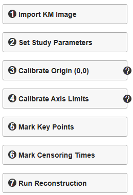
1. Import KM Image
First, acquire the target Kaplan-Meier curve from the published study (e.g., using a high-resolution screen capture) and save it locally. Then, click the "Import KM Image" button to load the file. Upon a successful import, the image will be rendered in the main canvas area, allowing users to identify a target curve and proceed with Steps 2–7 for IPD reconstruction.
2. Set Study Parameters
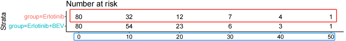
This step involves configuring the study parameters, including the At-risk Table, Sample Size, Number of Events, and Group Name. Note that Sample Size and Group Name are mandatory fields. If the At-risk Table is reported in the published study, users should input the time intervals and corresponding number at risk for the specific curve being reconstructed.
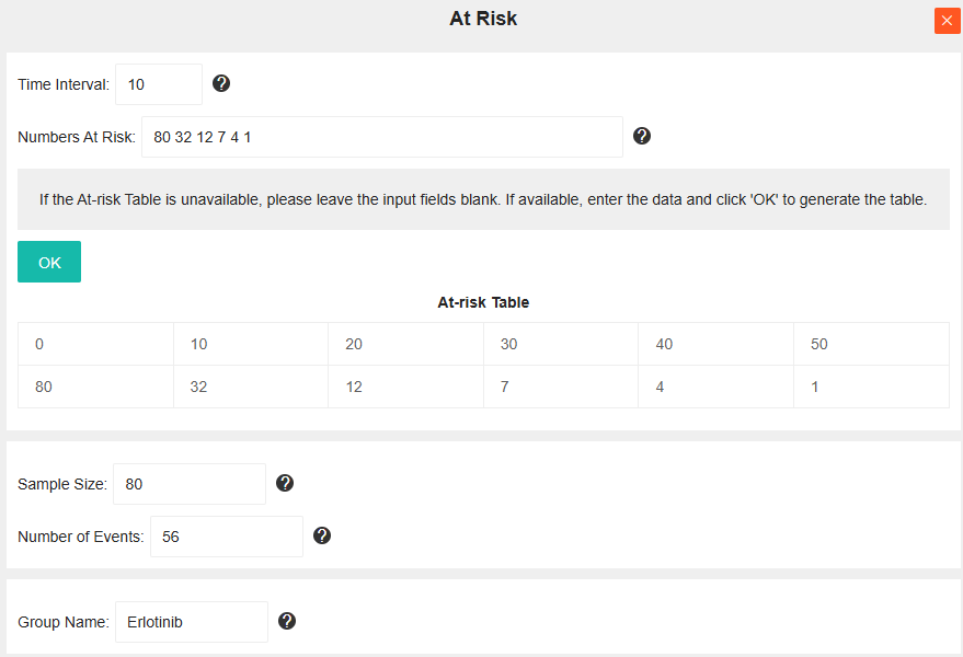
Example Workflow: To reconstruct the IPD for the Erlotinib group (see figure below), first input the At-risk data. Given the time points [0, 10, 20, 30, 40, 50] and risk counts [80, 32, 12, 7, 4, 1]:
- Enter "10" in the "Time Interval" field.
- Enter "80 32 12 7 4 1" (space-separated) in the "At Risk Num" field.
- Click "OK" to automatically generate the At-risk Table. The Sample Size field will be auto-populated based on the count at time 0.
- Finally, input the "Number of Events" (If the Number of Events is not available, please retain the default value of 0.) and "Group Name", then close the window to complete Step 2.
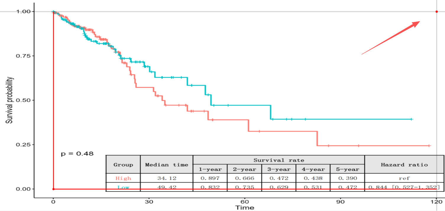
3. Calibrate Origin (0,0)
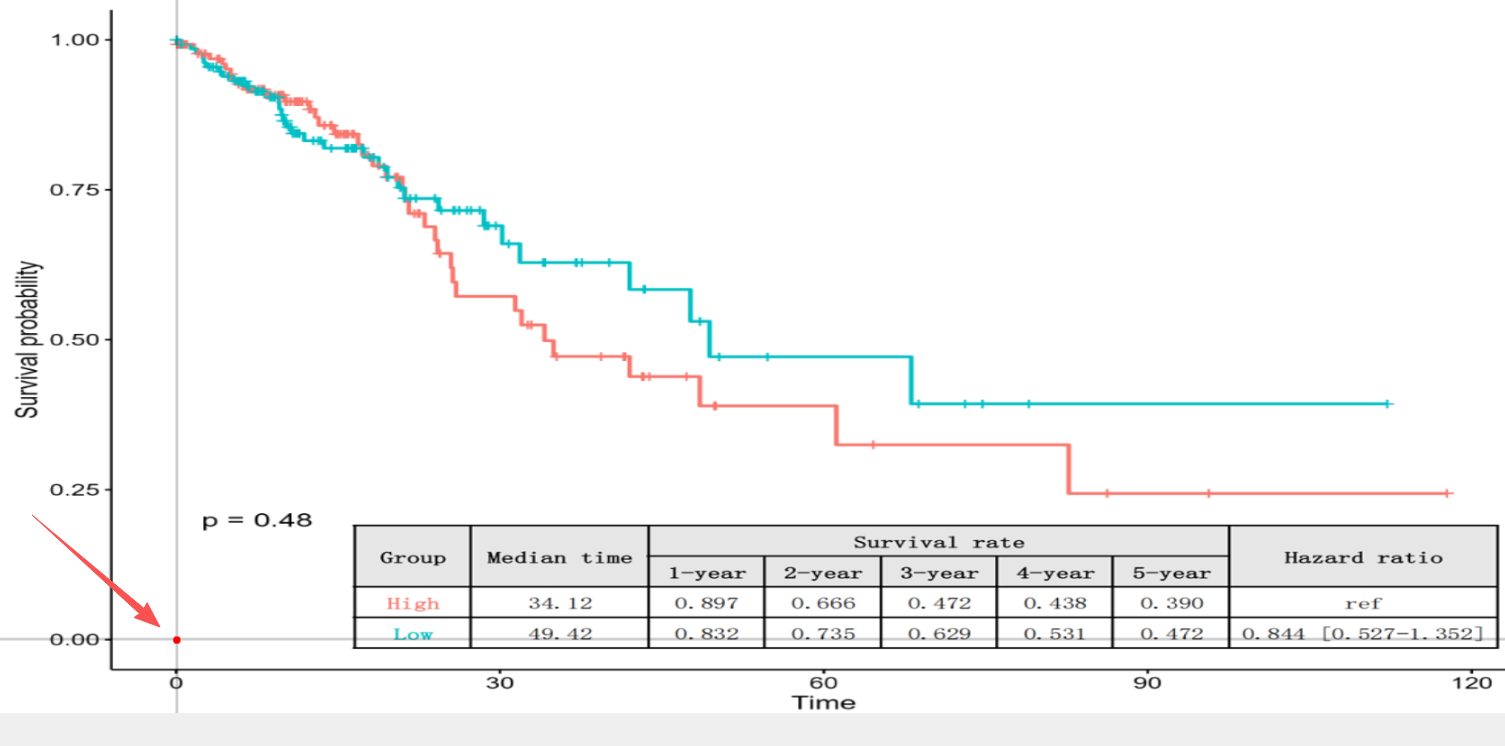
To establish the coordinate system, click the "Calibrate Origin (0,0)" button to activate the tool. Then, precisely click the origin point (0,0) on the KM curve image. The selected location will be visualized as a red dot.
Note: Ensure the coordinate origin is accurately placed. While usually located at the intersection of the Time axis and the Survival probability axis, the origin may be offset in certain publication styles (as illustrated below). If misaligned, click again to reposition the point.
4. Calibrate Axis Limits
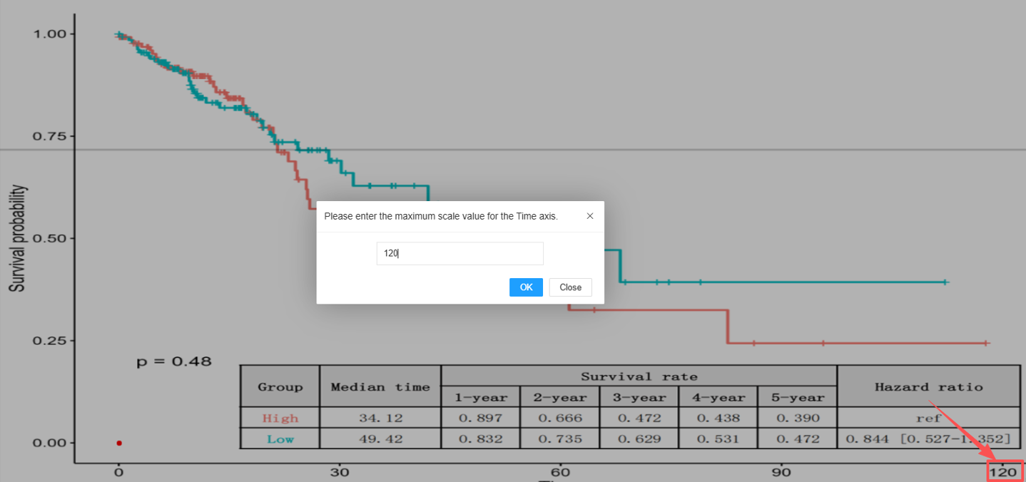
Click the "Calibrate Axis Limits" button to initiate the process.
- Input Value: A dialog box will appear. Enter the numerical value corresponding to the maximum Time axis limit (e.g., the largest time point marked on the axis) and click "OK".
- Mark Coordinate: Click the point representing the intersection of the maximum Time axis scale and the Survival probability axis scale of 1.0 (100% survival).
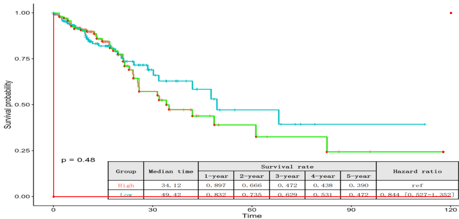
5. Mark Key Points
Basic Operation: The starting point at t = 0 is automatically locked to a survival probability of 1.0. Select the subsequent key point along the curve to begin. KM-PoPiGo generates a real-time reconstruction overlay, allowing for instant verification against the original KM image.Interactive Editing & Smart Correction:
- Add Point: Left-click to add a new key point.
- Delete Point: Right-click on an existing point to remove it.
- Auto-Correction: Points violating KM constraints (e.g., monotonicity) are automatically adjusted by the algorithm. Therefore, users need only focus on maximizing the visual overlap (fidelity) between the real-time curve and the original KM image.
Special Instructions for Endpoints:
- Horizontal Endpoint (Censoring): If the curve ends horizontally, click above the previous point.
- Zero Survival Endpoint: If the curve drops to zero, click below the Time axis (auto-clamped to 0).
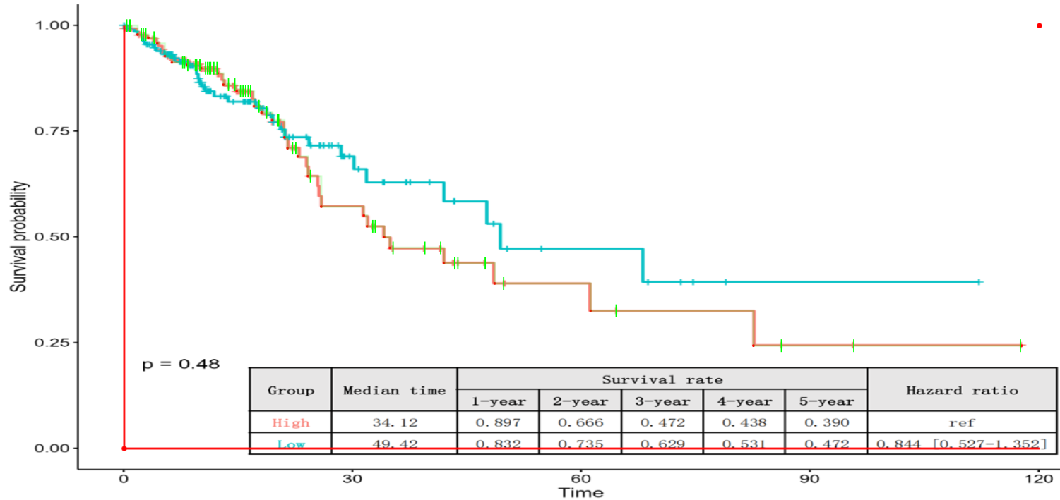
6. Mark Censoring Times
If the published curve visualizes censoring events (typically shown as vertical tick marks or crosses), click the "Mark Censoring Times" button to record them. Interactive Editing:
- Add Mark: Left-click on the censoring mark on the curve.
- Delete Mark: Right-click on an existing mark to remove it.
Crucial Note on Data Reliability: Users should exercise caution and only mark censoring events that are clearly distinguishable. If a mark is ambiguous or blurred due to image quality, it is preferable to omit it to maintain the statistical integrity of the reconstruction.
7. Run Reconstruction
Initiate the core calculation by clicking the "Run Reconstruction" button. The tool employs a genetic optimization algorithm to iteratively infer event times and censoring distributions for each time interval. Performance Note: The computational duration scales with data complexity. A larger total sample size or an increased number of marked points will naturally require more processing time to reach convergence.
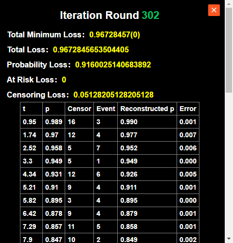
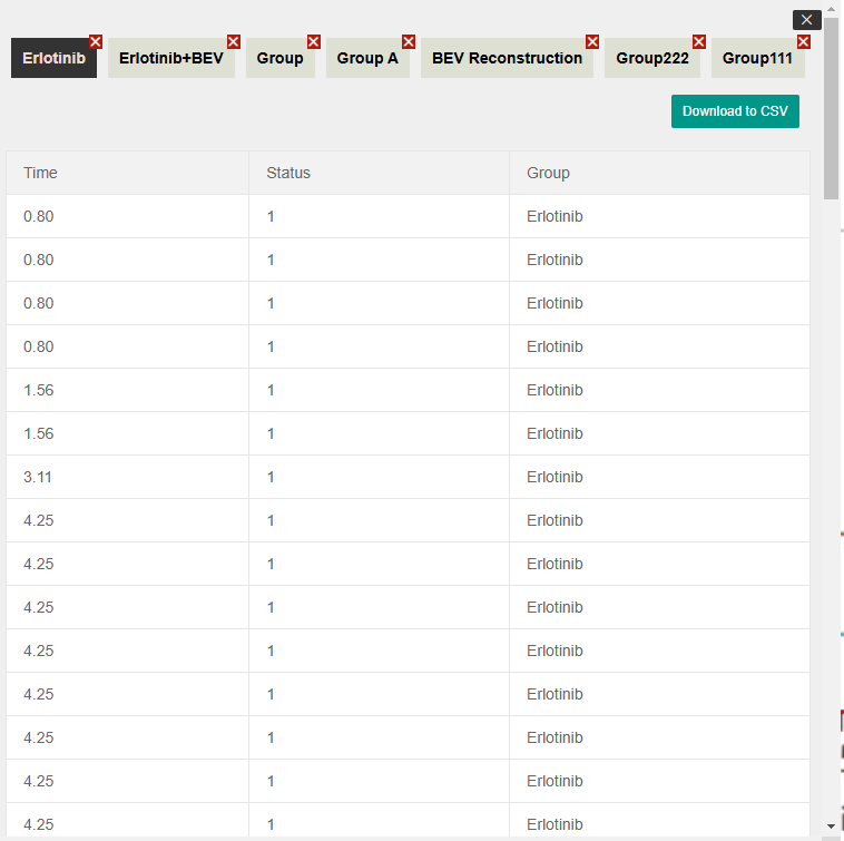
Reconstruction Results & Data Export
Upon the completion of the reconstruction algorithm, the generated datasets are automatically archived in the "Reconstruction Results" module. By navigating to this section, users can access a central repository of all processed Kaplan-Meier curves.
Key functionalities in this module include:
- Data Review: Inspect the detailed Individual Patient Data (IPD) generated for each session.
- Record Management: Delete obsolete or incorrect historical records to maintain a clean workspace.
- Data Export: Download the specific IPD datasets as standard CSV files, ready for downstream statistical analysis (e.g., in R, SPSS, or Python).
Generate R Code
KM-PoPiGo facilitates seamless downstream analysis by providing automated generation of commonly used R scripts. Access this interface by clicking the "Generate R Code" button. Supported analyses include:
- Hazard Ratio (HR) Calculation
- Median & Survival Rate (Median Survival Time and Survival Rate)
- Kaplan-Meier Curve Plotting
Configuration Rules: The Median & Survival Rate function is designed for single-group analysis. In contrast, the Hazard Ratio and KM Plotting functions support multi-group comparisons. When generating Hazard Ratio scripts, a Reference Group must be explicitly selected.
Adaptive Data Integration: The tool intelligently formats the output based on sample size:
- Small Sample Size: The IPD data is directly embedded within the R script. Users can simply copy and paste the code into R for immediate execution without external dependencies.
- Large Sample Size: To maintain code readability and performance, the script is generated to load the IPD via CSV. Ensure the corresponding data file is saved in your R working directory.
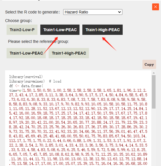
For example, if we select the Erlotinib and Erlotinib+BEV groups to generate R code, and choose Erlotinib as the reference group, the following code will be generated:
library(survival)
library(survminer)
df <- data.frame(
time=c(1.84,1.84,0.92,2.88,2.36,3.92,3.92,5.00,5.00,5.71,5.71,5.71,5.71,5.36,6.60,6.60,6.60,6.15,7.26,7.26,6.76,6.93,7.09,8.49,9.25,10.14,10.14,10.14,10.14,10.14,9.70,10.80,10.80,11.89,11.89,11.35,12.55,12.55,12.55,13.25,13.25,13.25,12.90,13.92,13.59,14.67,14.67,15.28,15.28,16.84,15.80,16.32,18.68,18.68,18.68,18.68,18.68,20.05,20.05,20.94,20.94,22.31,23.87,23.87,23.09,25.14,25.80,26.65,26.08,26.37,29.15,27.27,27.90,28.52,30.85,32.17,42.12,37.14,46.81,51.51,0.80,0.80,0.80,0.80,1.56,1.56,3.11,4.25,4.25,4.25,4.25,4.25,4.25,4.25,4.25,3.30,3.49,3.68,3.87,4.06,4.86,4.86,4.86,5.38,5.38,5.38,5.38,6.65,6.65,6.65,7.22,7.22,7.22,8.25,8.25,8.25,8.68,8.68,9.20,9.20,9.20,9.20,8.94,9.58,9.58,9.58,9.58,9.58,10.42,10.42,10.42,10.42,11.42,10.92,13.82,13.82,13.82,13.82,12.62,15.80,15.80,15.80,15.80,15.80,15.80,14.81,17.74,18.82,20.00,23.58,26.23,27.55,29.29,31.98,34.01,38.40,46.18,40.99,43.59,55.66),
status=c(1,1,0,1,0,1,1,1,1,1,1,1,1,0,1,1,1,0,1,1,0,0,0,1,1,1,1,1,1,1,0,1,1,1,1,0,1,1,1,1,1,1,0,1,0,1,1,1,1,1,0,0,1,1,1,1,1,1,1,1,1,1,1,1,0,1,1,1,0,0,1,0,0,0,1,1,1,0,0,0,1,1,1,1,1,1,1,1,1,1,1,1,1,1,1,0,0,0,0,0,1,1,1,1,1,1,1,1,1,1,1,1,1,1,1,1,1,1,1,1,1,1,0,1,1,1,1,1,1,1,1,1,1,0,1,1,1,1,0,1,1,1,1,1,1,0,1,1,1,1,1,1,1,1,1,1,1,0,0,0),
group=c("Erlotinib+BEV","Erlotinib+BEV","Erlotinib+BEV","Erlotinib+BEV","Erlotinib+BEV","Erlotinib+BEV","Erlotinib+BEV","Erlotinib+BEV","Erlotinib+BEV","Erlotinib+BEV","Erlotinib+BEV","Erlotinib+BEV","Erlotinib+BEV","Erlotinib+BEV","Erlotinib+BEV","Erlotinib+BEV","Erlotinib+BEV","Erlotinib+BEV","Erlotinib+BEV","Erlotinib+BEV","Erlotinib+BEV","Erlotinib+BEV","Erlotinib+BEV","Erlotinib+BEV","Erlotinib+BEV","Erlotinib+BEV","Erlotinib+BEV","Erlotinib+BEV","Erlotinib+BEV","Erlotinib+BEV","Erlotinib+BEV","Erlotinib+BEV","Erlotinib+BEV","Erlotinib+BEV","Erlotinib+BEV","Erlotinib+BEV","Erlotinib+BEV","Erlotinib+BEV","Erlotinib+BEV","Erlotinib+BEV","Erlotinib+BEV","Erlotinib+BEV","Erlotinib+BEV","Erlotinib+BEV","Erlotinib+BEV","Erlotinib+BEV","Erlotinib+BEV","Erlotinib+BEV","Erlotinib+BEV","Erlotinib+BEV","Erlotinib+BEV","Erlotinib+BEV","Erlotinib+BEV","Erlotinib+BEV","Erlotinib+BEV","Erlotinib+BEV","Erlotinib+BEV","Erlotinib+BEV","Erlotinib+BEV","Erlotinib+BEV","Erlotinib+BEV","Erlotinib+BEV","Erlotinib+BEV","Erlotinib+BEV","Erlotinib+BEV","Erlotinib+BEV","Erlotinib+BEV","Erlotinib+BEV","Erlotinib+BEV","Erlotinib+BEV","Erlotinib+BEV","Erlotinib+BEV","Erlotinib+BEV","Erlotinib+BEV","Erlotinib+BEV","Erlotinib+BEV","Erlotinib+BEV","Erlotinib+BEV","Erlotinib+BEV","Erlotinib+BEV","Erlotinib","Erlotinib","Erlotinib","Erlotinib","Erlotinib","Erlotinib","Erlotinib","Erlotinib","Erlotinib","Erlotinib","Erlotinib","Erlotinib","Erlotinib","Erlotinib","Erlotinib","Erlotinib","Erlotinib","Erlotinib","Erlotinib","Erlotinib","Erlotinib","Erlotinib","Erlotinib","Erlotinib","Erlotinib","Erlotinib","Erlotinib","Erlotinib","Erlotinib","Erlotinib","Erlotinib","Erlotinib","Erlotinib","Erlotinib","Erlotinib","Erlotinib","Erlotinib","Erlotinib","Erlotinib","Erlotinib","Erlotinib","Erlotinib","Erlotinib","Erlotinib","Erlotinib","Erlotinib","Erlotinib","Erlotinib","Erlotinib","Erlotinib","Erlotinib","Erlotinib","Erlotinib","Erlotinib","Erlotinib","Erlotinib","Erlotinib","Erlotinib","Erlotinib","Erlotinib","Erlotinib","Erlotinib","Erlotinib","Erlotinib","Erlotinib","Erlotinib","Erlotinib","Erlotinib","Erlotinib","Erlotinib","Erlotinib","Erlotinib","Erlotinib","Erlotinib","Erlotinib","Erlotinib","Erlotinib","Erlotinib","Erlotinib","Erlotinib")
)
survival_data <- Surv(time = df$time, event = df$status)
fit <- coxph(survival_data ~ group, data = df)
df$group <- as.factor(df$group)
df$group <- relevel(df$group, ref = "Erlotinib")
summary_info <- summary(fit)
hr <- summary_info$conf.int[1, "exp(coef)"]
lhr <- summary_info$conf.int[1, "lower .95"]
rhr <- summary_info$conf.int[1, "upper .95"]
print(paste(round(hr,3),"[",round(lhr,3),"-",round(rhr,3),"]"))
The generated code above can be directly executed in R to obtain the Hazard Ratio for the specified groups.
Note on Data Loading: The system has automatically optimized the script based on sample size. If the code is generated to load data via an external file (for large datasets), please ensure you have downloaded the corresponding IPD .csv file from the "Reconstruction Results" module and placed it in your R working directory before execution.
library(survival)
library(survminer)
# Load CSV files
df1 <- read.csv("The directory where the Erlotinib.csv file is located/Erlotinib+BEV.csv",header=TRUE) #For example, D:/project/Erlotinib+BEV.csv
df2 <- read.csv("The directory where the Erlotinib.csv file is located/Erlotinib.csv",header=TRUE) #For example, D:/project/Erlotinib.csv
# Combine the loaded groups into a single dataframe
df <- rbind(df1,df2)

df$group <- as.factor(df$group)
# Note: Modify the reference group name below
df$group <- relevel(df$group, ref = "Erlotinib")

survival_data <- Surv(time = df$time, event = df$status)
fit <- coxph(survival_data ~ group, data = df)

summary_info <- summary(fit)
hr <- summary_info$conf.int[1, "exp(coef)"]
lhr <- summary_info$conf.int[1, "lower .95"]
rhr <- summary_info$conf.int[1, "upper .95"]
print(paste(round(hr,3),"[",round(lhr,3),"-",round(rhr,3),"]"))